Zero Knowledge Proof: Polynomial Commitments based on Error-correcting Codes
Table of Contents
In this post, we will talk about other polynomial commitment scheme based on Error-correcting codes.
Resources
Poly-commits: Error-Correcting Codes - Cryptonotes
Background
Error-correcting code
An error-correcting code encodes a message of length $k$ into a codeword of length $n$, where $n > k$. The minimum distance (which is well-known as Hamming distance) between any two codewords is shown as $\Delta$. These parameters are important, and we may refer to an error-correcting code as $[n, k, \Delta]$ code.
For example, let’s take a look at repetition code: $[6, 2, \Delta = 3]$
Enc(00) = 000000, Enc(01) = 000111
Enc(10) = 111000, Enc(11) = 111111
We can correct 1 error during the transmission, e.g. 010111 -> 01, and we define Dec(c) is the decode algorithm.
Rate and relative distance
With $[n, k, \Delta]$ code, we introduce some terminologies:
- Rate: Define as $\frac{k}{n}$
- relative distance: Define as $\frac{\Delta}{n}$
E.g. repetition code with rate $\frac{1}{a}, \Delta = a$, relative distance $\frac{1}{k}$.
We want both rate and relative distance can be as high as possible, but generally there is a trade-off between them.
Linear code
Linear code is a common code with a requirement: any linear combination of codewords is also a codeword.
Therefore, encoding can always be represented as vector-matrix multiplication between $m$ and the generator matrix.
A thing to keep in mind is that the minimum distance is the same as the codeword with the least number of non-zeros (which is called weight)
Reed-Solomon Code
Reed-Solomon is a widely used error-correcting code.
- The message is viewed as a unique degree $k - 1$ univariate polynomial
- The codeword is the evaluations at $n$ points. For example, the codeword can be $(\omega, \omega^2, …, \omega^n)$ for $n$-th root-of-unity $\omega$, where $\omega^n = 1 \mod p$
- The distance $\Delta = n - k + 1$. This is the best choice we can have because:
- A degree $k - 1$ polynomial has at most $k - 1$ roots
- Since the codeword is $n$ evaluations, we subtract the number of roots from this to get the minimum number of non-zeros
- Encoding time is $\mathcal{O}(n \log n)$ using FFT
For $n = 2k$, the rate is $\frac{1}{2}$ and relative distance is $\frac{1}{2}$.
Polynomial commitment based on linear code
Polynomial coefficients in a matrix
To begin constructing our poly-commit scheme, we will first take a different approach on representing our polynomial. Remember that there was a “coefficient representation” where we simply stored the list of coefficients as a vector. Now, we will use a matrix to do that.
Suppose that you have a polynomial $f(x)$ where $\deg(f) = d$ is a perfect square (note that if $d$ is not square, we can pad the polynomial by adding higher monomial with zero coefficient), we can write our polynomial as $$f(x) = \sum_{i=1}^{\sqrt{d}} \sum_{j = 1}^{\sqrt{d}} f_{i, j}u^{i - 1 + (j - 1) \sqrt{d}}$$
With the representation below, we can rewrite the coefficients by the following matrix:
$$\begin{pmatrix} f_{1, 1} & f_{1, 2} & \dots & f_{1, \sqrt{d}} \newline f_{2, 1} & f_{2, 2} & \dots & f_{2, \sqrt{d}} \newline \vdots & \vdots & \ddots & \vdots \newline f_{\sqrt{d}, 1} & f_{\sqrt{d}, 2} & \dots & f_{\sqrt{d}, \sqrt{d}} \end{pmatrix}$$
Evaluation of this polynomial at some point $u$ can then be shown as some matrix-vector multiplication:
$$f(u) = [1, u, u^2, …, u^{\sqrt{d} - 1}] \times \begin{pmatrix} f_{1, 1} & f_{1, 2} & \dots & f_{1, \sqrt{d}} \newline f_{2, 1} & f_{2, 2} & \dots & f_{2, \sqrt{d}} \newline \vdots & \vdots & \ddots & \vdots \newline f_{\sqrt{d}, 1} & f_{\sqrt{d}, 2} & \dots & f_{\sqrt{d}, \sqrt{d}} \end{pmatrix} \times \begin{bmatrix} 1 \newline u^{\sqrt{d}} \newline u^{2 \sqrt{d}} \newline \vdots \newline u^{d - \sqrt{d}} \end{bmatrix}$$
And with this, we will be able to reduce a polynomial commitment of proof size $\sqrt{d}$ to an argument for vector-matrix product into as shown below:
$$[1, u, u^2, …, u^{\sqrt{d} - 1}] \times \begin{pmatrix} f_{1, 1} & f_{1, 2} & \dots & f_{1, \sqrt{d}} \newline f_{2, 1} & f_{2, 2} & \dots & f_{2, \sqrt{d}} \newline \vdots & \vdots & \ddots & \vdots \newline f_{\sqrt{d}, 1} & f_{\sqrt{d}, 2} & \dots & f_{\sqrt{d}, \sqrt{d}} \end{pmatrix} = \underbrace{[\dots]}_{\sqrt{d}}$$
The prover could send this resulting vector to the verifier, and the verifier could evaluate the second step locally by using column vector made of $u$ which the verifier knows. By this way, the commitment size of degree $d$ polynomial is reduced to $\sqrt{d}$.
The problem now is to somehow convince the verifier that the prover has used the correct coefficients in the 2D matrix. For that, the prover does the following:
- Transform the $\sqrt{d} \times \sqrt{d}$ matrix into a $\sqrt{d} \times n$ matrix, where each row of length $\sqrt{d}$ is encoded into a codeword of length $n$ using a linear code
- The resulting $\sqrt{d} \times n$ matrix is committed using a Merkle Tree, where each column is a leaf
- The public parameter is just made of the decided Hash function to be used in Merkle Tree, so there is no trusted setup required.
With that said, the entire algorithm can be split into two steps:
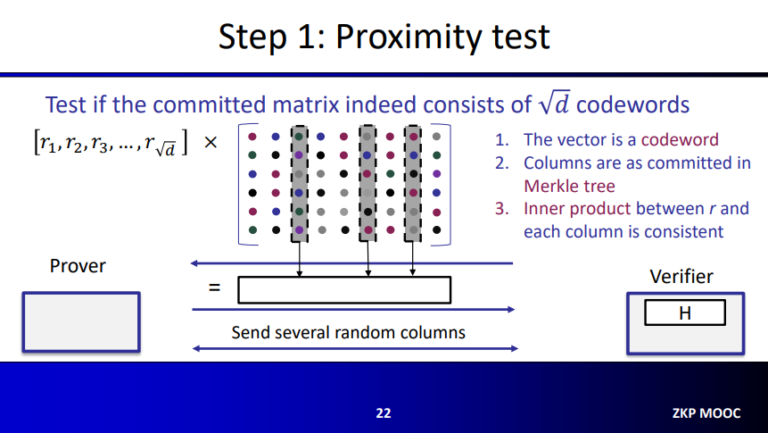
Proximity Test
For the proximity test, the Verifier sends a random vector $\overrightarrow{r} = [r_1, r_2, …, r_{\sqrt{d}}]$ with size $\sqrt{d}$. Then the prover multiplies the vector with the matrix (size $\sqrt{d} \times n$) to obtain another vector of size $n$. Afterwards, the verifier asks to reveal several columns of this matrix, and the prover reveals them.
With that, the verifier checks the following:
- The resulting vector is a codeword, which should be true because any linear combination of codeword is a codeword.
- Columns are as committed in the Merkle Tree.
- Inner product between $\overrightarrow{r}$ and each column is consistent, this is done simply by looking at the corresponding elements in the size $n$ vector.
If all these are correct, then the proximity test is passed with overwhelming probability.
Soundness
To get an intuition, suppose the prover cheats, then we have two possible positions:
If he tries to use a different matrix, by the linear property of codewords, the resulting vector will not be a codeword. The first check ensures this.
If somehow prover pass the first check, the matrix still has many different locations from the correct answer. The second check ensures that columns are as committed.
If prover use the correct matrix but send a different result vector, then he can’t pass third check due to properties of Reed-Solomon.
For a formal form, a new parameter $e$ is introduced. For $e < \frac{\Delta}{4}$, if the commited matrix $C$ is $e$-far from any codeword (meaning that the minimum distance of all rows to any codeword in the linear code is at least $e$), then $$\Pr{[\omega = r^TC \ is \ e-close \ to \ any \ codeword ]} \le \frac{e+1}{\mathbb{F}}$$
So, if $\omega = r^TC$ is $e$-far from any codeword then finally: $$\Pr{[Check \ 3 \ passes \ for \ t \ random \ columns]} \le (1 - \frac{e}{n})^t$$
Discovery
This test was discovered independently by the two papers:
Ligero [AHIV'2017]: Interleaved test. Reed-Solomon code
[BCGGHJ'2017]: Ideal linear commitment model with linear-time encodable code -> first SNARK with linear prover time
Optimization
The prover can actually send a message $m$ instead of the size $n$ result vector, such that the encoding of $m$ is equal to the codeword that is the resulting vector. This is good because:
- The message with size $\sqrt{d}$ is smaller than the vector of size $n$
- Check 1 is implicity passed
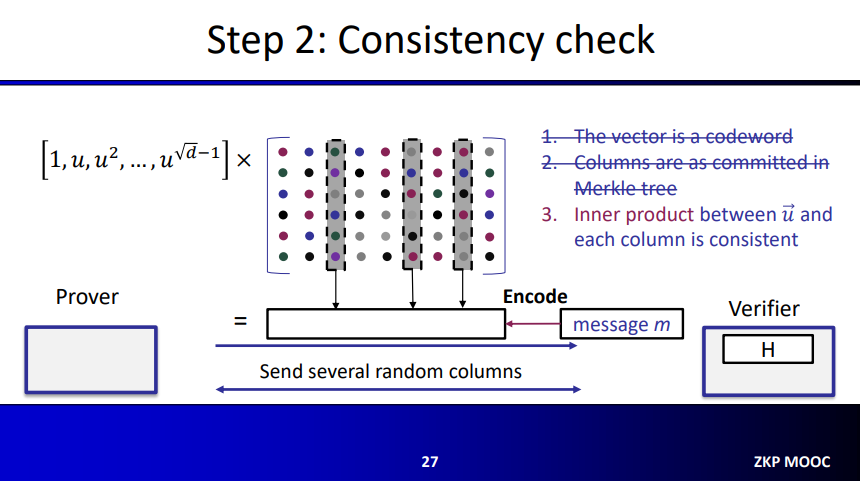
Consistency Test
The algorithm for consistency test is almost the same as the optimized proximity test. The prover sends a message $m$, which is the multiplication of $\overrightarrow{u}$(that is $f(u)$) with the coefficient matrix $C$. Then, the verifier finds the encoding of this message.
Columns are ensured to be the committed ones, because we have already made that check in the proximity test. Furthermore, using the same randomly picked columns (corresponding to elements in the codeword) the verifier will check whether the multiplication is consistent.
In short:
- The resulting vector is a codeword, true because vector was created from the encoding of $m$.
- Columns are as committed in the Merkle Tree, true because this was done in the previous test.
- Inner product between $\overrightarrow{u}$ and each column is consistent. which is checked using the same randomly picked columns (for efficiency)
Soundness (intuition)
- By the proximity test, the committed matrix $C$ is close to a codeword.
- There exists an extractor that extracts $F$ by Merkle tree commitment and decoding $C$, such that $\overrightarrow{u} \times F = m$ with probability $1 - \epsilon$
Polynomial commitment based on linear codes
With these tools above, we are ready to talk about the polynomial commitment based on linear codes.
- Keygen: Sample a hash function
- Hash function are public, so this is a transparent setup!
- $\mathcal{O}(1)$ complexity, transparent setup.
- Commit: Encode the coefficient matrix of $f$ row-wise with a linear code, compute the Merkle tree commitment.
- The complexity is $\mathcal{O}(d \log d)$ field multiplications using RS code, $\mathcal{O}(d)$ using linear-time encodable code
- For merkle tree, we have $\mathcal{O}(d)$ for hashed, and $\mathcal{O}(1)$ commitment size
- Eval and Verify:
- Proximity test: random linear combination of all rows, check its consistency with $t$ random columns
- Consistency test: $\overrightarrow{u} \times F = m$, encode $m$ and check its consistency with $t$ random columns
- $f(u) = \braket{m, \overrightarrow{u}’}$
- Eval take $\mathcal{O}(d)$ field operations, and can be made non-interactive using Fiat-Shamir
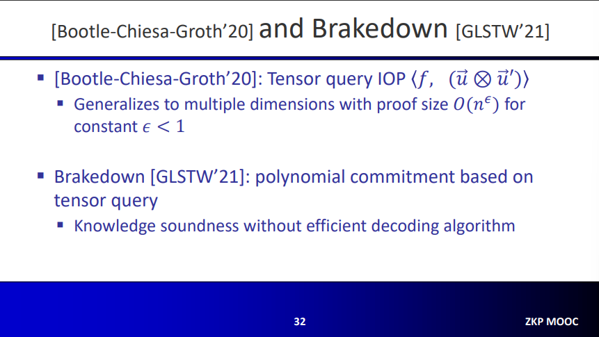
This method has proof size $\mathcal{O}(\sqrt{d})$ and verifier time $\mathcal{O}(\sqrt{d})$.
Practice
Linear-time encodable code
Expander Graphs
Expander graph is a graph that has strong connectivity properties, quantified using vertex, edge or spectral expansion. We use bipartite graph as an example: With bipartite graph, a graph that can be split in two parts such that no vertex within that sub-graph are connected.
We can use an expander as a linear code by let each vertex in the left correspond to symbols of the message $m$, and let the right side correspond to symbols of the codeword.
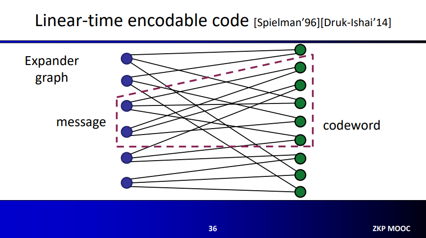
Note that this way is not sufficient; it fails on the “constant relative distance” requirement. Take a message with a single non-zero for example, the codeword must look the same for all such messages. Obviously, this is not the case here, because codewords symbols change depending on which symbol of the message is non-zero.
Lossless Expander Graph
Let $|L|$ be the number of vertices in the left graph, and set $|R| = \alpha |L|$ for some constant $\alpha$. In the example above, $\alpha$ is larger than 1, but in practice we actually have $0 < \alpha < 1 $. Let $g$ be the degree of a left node.
For every subset $S$ of nodes on the left, the maximum possible expansion is $g|S|$. Let $\varGamma$ denote the set of neighbors for a set, i.e. $|\varGamma(S)| = g|S|$. However, this is not true for all subset, and you need to satisfiy this constraint: $$|S| \le \frac{\alpha|L|}{g}$$
In practice, we use a more relaxed definition: We let the maximum expansion $|\varGamma(S)| \ge (1 - \beta)g|S|$ with the constraint $$|S| \le \frac{\delta|L|}{g}$$ for some $\delta$. In previous definition, we use $\beta = 0$ and $\delta = \alpha$.
Recursive Encoding Algorithm
Encoding Algorithm
Because lossless expander itself is not enough, we will do the encoding recursively. In this case, we will start with a message $m$ of length $k = |m|$ and finish with a codeword of size $4k$. This codeword is a combination of 3 parts:
- The message itself, length $k$
- Encoded message, using a lossless expander with $\alpha = 1/2$. The resulting code has size $k/2$. This result is then encoded using an existing (assumed) encoder of rate $1/4$. The resulting codeword has length $4 \times (k \ 2) = 2k$.
- Another encoded message with length $k$, is generated by using a lossless expander with $\alpha = 1/2$ to encode previous codeword.
$$codeword = m || c_1 || c_2$$
Recursive encoding
To become recursive, we can use the algorithm and repeat for $k/2$, $k/4$,… until a constant size, and use any code with good distance (e.g. Reed-Solomon) to do the encoding job.
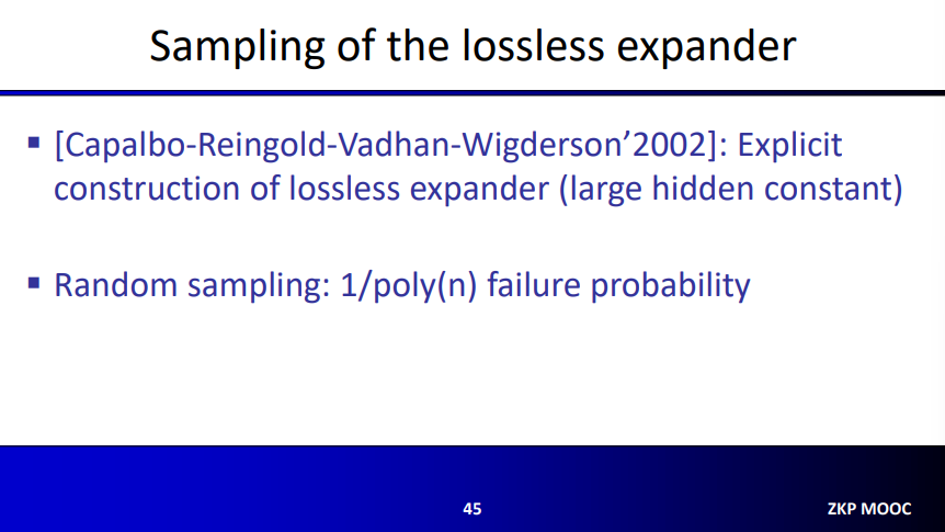
Sampling of the lossless expander
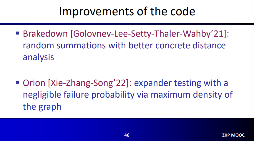
Improvements of the code
Summary
Polynomial commitment (and SNARK) based on linear code has the following properties:
- Transparent setup, $\mathcal{O}(1)$
- Commit and Prover times are $\mathcal{O}(d)$ field operations
- Plausibly post-quantum secure with Error-Correcting Code
- Field agnostic
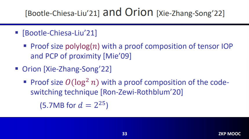
- Proof size is $\mathcal{O}(\sqrt{d})$, MBs, which is not good.