Zero Knowledge Proof: The PLONK SNARK
Table of Contents
In this posts, we will construct a widely used SNARK called PLONK
Resources
PLONK: Permutations over Lagrange-bases for Oecumenical Noninteractive arguments of Knowledge
Feist-Khovratovich technique for computing KZG proofs fast
Detail
Recall: Polynomial Commitment
If you don’t know anything about polynomial commitment, I suggest reading my previous post. Here is a short explanation about what they are:
The prover would like to commit to some polynomial $f \in \mathbb{F}_p^{\le d}[X]$
An $eval$ finction uses evaluate some values for this polynomial, without revealing it. For example, pick some public $u, v \in \mathbb{F}_p$
Prover will convince that $f(u) = v$ and $deg(f) \le d$
Verifier will only know $d, u, v$ and a polynomial commitment $comm_f$, also shown as $f$ sometimes
The proof size for $eval$ and the verifier time should both be in $\mathcal{O}_{\lambda}(\log d)$
The KZG polynomial commitment scheme
Let’s talk about KZG [Kate-Zaverucha-Goldberg'10] polynomial commitment scheme. We will work with finite cyclic group $\mathbb{G}$ of order $p$ with generator $g$
Trusted Setup: $setup(\lambda) \to gp$
KZG starts with a trusted setup $setup(\lambda) \to gp$ to produce public parameters. This is done as follows:
Sample some random $\tau \in \mathbb{F}_p$
Calculate public parameters $gp$: $$gp = (H_0 = g, H_1 = \tau g,..,H_d = \tau^d g) \in \mathbb{G}^{d+1}$$
and we will have $|gp| = d + 1$
- Delete $\tau$. If this number is leaked and in wrong hands, they can create fake proofs. This is why the setup must take place in a trusted environment.
Commitment: $commit(gp, f) \to comm_f$
A commitment will take the public parameters $gp$ along with the polynomial $f$ to be committed, and produces the commitment
The commitment is shown as $commit(gp, f) \to comm_f$
Our commitment will be $comm_f = f(\tau)g \in \mathbb{G}$
How to calculate $f(\tau)$ without knowledge of $\tau$?. Let’s take a look about the function $f$: $$f(X) = f_0 + f_1X + f_2X^2 + … + f_dX^d$$
Remember that we know $H_i = X^i, i = 0..d$, so we can calculate: $$f_0 H_0 + f_1 H_1 + … + f_d H_d$$
When you expand $H_i$, you will see that: $$f_0g + f_1 \tau g + f_2 \tau^2 g + … + f_d \tau^d g = f(\tau)g$$
And you get the commitment you want! Note that this commitment is binding but not hiding as is.
Evaluation: $eval$
Let us now see how a verifier evaluates the commitment
Prover knows $(gp, f, u, v)$ and wants to prove that $f(u) = v$
Verifier knows $(gp, comm_f, u, v)$
We will use some well-known properties of polynomial:
$f(u) = v$ if and only if $u$ is a root of $\hat{f} = f - v$.
$u$ is a root of $\hat{f}$ if and only if the polynomial $(X - u)$ divides $\hat{f}$
$(X - u)$ divides $\hat{f}$ if and only if $\exist q \in \mathbb{F}_p[X]$ such that $q(X)(X - u) = \hat{f}(X) = f(X) - v$. This is another way of saying that since $(X - u)$ divides $\hat{f}$ there will be no remainder left from this division, and there will be some resulting quotient polynomial $q$
Now we can talk about the plan:
Prover computes $q(X)$ and commits to $q$ as $comm_q$. Remember that commitment results in a single group element only
Prover send the proof $\pi = comm_q$
Verifier accepts if $(\tau - u) comm_q = comm_f - vg$
You can see the appearance of $\tau$ here, which is supposed to be secret. Well, we use pairing to hide $\tau$ while still allowing the above computation. In doing so, only $H_0$ and $H_1$ will be used, which makes this thing independent of degree $d$
Actually, we still need $d$. The prover must compute the quotient polynomial $q$ and the complexity of that is related to $d$, so you will lose from prover time when you have large degrees
To prove that this is a secure poly-commit scheme, we need to dig deeper about polynomial commitments, which will be described in my next post
Properties of KZG
Generalizations: It has been shown that you can use KZG to commit to $k$-variate polynomials
Batch Proofs: Suppose you have commitments to $n$ polynomials $f_1, f_2, …, f_n$ and you have $m$ values to reveal in each of them, meaning that you basically want to prove all evaluations defined by $f_i(u_{i,j}) = v_{i, j}$ for $i \in [n]$ and $j \in [m]$. Normally, this would require $n \times m$ evaluations, but thanks to KZG we can actually do this in a single proof that is a single group element
Linear-time Commitments: We have several ways to represent a polynomial $f(X)$ in $\mathbb{F}_p^{(\le d)}[X]$:
Coefficient representation: We will store $f(X) = f_0 + f_1X + … + f_dX^d$ as an array of values $[f_0, f_1,…,f_d]$. So we can compute the commitment in linear time $\mathcal{O}(d)$ since we just have to multiply $f_i$ with $H_i$ for $i \in [d]$, giving us $comm_f = f_0H_0 + f_1H_1 + … + f_dH_d$
Point-value representation with NTT(Number Theoristic Transfrom): A polynomial of degree $d$ can be defined by $d + 1$ points. So we have $d + 1$ points: $(a_0, f(a_0)), (a_1, f(a_1)),…,(a_d, f(a_d))$
To compute $comm_f$ naively, we can construct the coefficients $f_0, f_1, …,f_d$ to basically convert point-value representation to coefficient representation, then compute the commitment
We can use Number Theoretic Transfrom (NTT), which is closely related to Fourier Transform, to convert from point-value to coefficient representation. The complexity is $\mathcal{O}(d \log d)$
Point-value representation with Lagrange Interpolation:
We can use Lagrange Interpolation to speed up our commitment computing! So we have: $$\begin{aligned} f(\tau) &= \sum _ {i=0}^{d} \lambda _ i(\tau) f(a _ i) \newline \lambda _ i (\tau) &= \frac{\prod ^ d _ {j = 0, j \ne i} (\tau - a_j)}{\prod ^ d _ {j = 0, j \ne i} (a_i - a_j)} \in \mathbb{F}_p \end{aligned}$$
The idea here is that our public parameters will actually be in Lagrange form, and the process of getting this just a linear transformation that everyone can do. So, we obtain public parameter $\hat{gp}$ that looks like: $$\hat{gp} = (\hat{H}_0 = \lambda_0(\tau)g, \hat{H}_1 = \lambda_1(\tau)g, …, \hat{H}_d = \lambda_d(\tau)g) \in \mathbb{G}^{d+1}$$ This way, the commitment can be compute in linear time $\mathcal{O}(d)$: $$comm_f = f(\tau)g = f(a_0)\hat{H}_0 + f(a_1)\hat{H}_1 + … + f(a_d)\hat{H}_d$$
KZG fast multi-point proof generation
Let $\Omega \subseteq \mathbb{F}_p$ and $|\Omega| = d$. Suppose that the prover needs an evaluation proofs $\pi_a \in G$ for all $a \in \Omega$
With a naive way, this takes time $\mathcal{O}(d^2)$, because $d$ proofs each takes time $\mathcal{O}(d)$
Thankfully, we can use Feist-Khovratovich'23 to do this: If $\Omega$ is a multiplicative subgroup, the evaluation takes time in $\mathcal{O}(d \log d)$, otherwise, it takes time in $\mathcal{O}(d \log^2 d)$
Dory Poly-commit Scheme
We have some difficulties with KZG:
Requires a trusted setup to compute the public parameters $gp$
$gp$ size is linear in the degree $d$
To deal with that hurdle, we can use Dory Lee'20. It has some properties:
Transparent setup: No secret randomness in setup
$comm_f$ is a single group element, independent of degree
$eval$ proof size for $f \in \mathbb{F}_p^{\le d}[X]$ is $\mathcal{O}(\log d)$ group element, while KZG’s $eval$ proof size is constant
$eval$ verify time is $\mathcal{O}(\log d)$, KZG took constant time
prover time is $\mathcal{O}(d)$
PCS to Commit to a Vector
We will talk about vector commitment, which is a drop-in replacement for Merkle Trees
Suppose that Bob want to commit a vector $(u_1, …, u_k) \in \mathbb{F}_p^{(\le d)}$. He can interpolate a polynomial $f$ such that $f(i) = u_i$ for $i = 1,..,k$ and commit $f$ as we have described above
If Alice wants to query some elements like “show me that $u_2 = a$ and $u_4 = b$”, it is equivalent to “show me $f(2) = a$ and $f(4) = b$” and we know we can prove this in a single group element using batch proof, which is a very cool property of KZG
When we use a Merkle Tree, each evaluation proof would have size $\mathcal{O}(\log k)$ and for $l$ proofs this would mean $\mathcal{O}(l \log k)$ proof size, a lot bigger than the constant proof size of KZG.
For more applications of using PCS in Merkle Trees, you can check Verkle Tree
Proving properties of committed polynomials
Notation:
When we say the verifier queries a polynomial $f$ at some random point $r$ to get $f(r)$, we actually mean that the prover computes $y = f(r)$ and a proof of this evaluation $\pi_f$, then it sends back $y, \pi_f$ to the verifier
Everything we will do in our interactive proofs will be public-coin protocols, so we can compile it into non-interactive protocols using Fiat-Shamir
Equality Testing
In KZG, to test if $f = g$, verifier only need to know $comm_f, comm_g$. But this isn’t enough for more complex equality tests
For example, suppose that the verifier want to see if $f = g_1 g_2 g_3$ and has $comm_f, comm_{g_1}, comm_{g_2}, comm_{g_3}$. The verifier need to query all four polynomial at random $r \in \mathbb{F}_p$ and test equality, and this takes lots of work !
Important Proof Gadgets for Univariates
Let $\Omega$ be some subset of $\mathbb{F}_p$ of size $k$
First, we need to know about the vanishing polynomial
Definition: The vanishing polynomial of $\Omega$ is $$ Z_{\Omega}(X) := \prod _ {a \in \Omega}(X - a)$$ with $deg(Z_{\Omega}) = k$
Then, let $\omega$ be a primitive $k$-th root of unity, meaning that $\omega^k = 1$. If the set $\Omega$ is defined as follows: $$\Omega = \lbrace 1, \omega, \omega^2,…, \omega^{k - 1} \rbrace \subseteq \mathbb{F} _ p$$ then $Z_{\Omega}(X) = X^k - 1$.
For $r \in \mathbb{F} _ p$, evaluating $Z_{\Omega}(r)$ takes $\le 2 \log _ 2 k$ field operations, thanks to multiply-and-square method
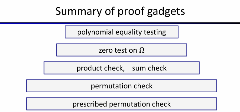
Now, we will construct efficient poly-IOPs for the following proof gadgets: Let $f, g \in \mathbb{F}_p^{(\le d)}[X]$ be polynomials of degree $d$ and $d \ge k$. The verifier has a commitment to these polynomials, $comm_f$ and $comm_g$. Our proof gadgets will have:
Equality Test: prove that $f, g$ are equal. We know that evaluating them at a random point and seeing if they are equal does the trick, assuming degree is much smaller than the size of the finite field.
Zero Test: prove that $f$ is identically zero on $\Omega$, meaning that it acts like a zero-polynomial for every value in $\Omega$, but of course it can do whatever it wants for values outside of $\Omega$ but in $\mathbb{F}_p$
Sum Check: prove that $\sum_{a \in \Omega}f(a) = 0$
Product Check: prove that $\prod_{a \in Omega}f(a) = 1$
Permutation Check: prove that evaluations of $f$ over $\Omega$ is a permutation of evaluations of $g$ over $\Omega$
Prescribed Permutation Check: prove that evaluations of $f$ over $\Omega$ is a permutation of evaluations of $g$ over $\Omega$, with a “prescribed” permutation $W: \Omega \to \Omega$. This permutation is a bijection $\forall i \in [k]: W(\omega^i) = \omega^j$
Zero Test
To understand Zero Test, we need to know about a simple but useful lemma
Lemma: $f$ is zero on $\Omega$ if and only if $f(X)$ is divisible by $Z_{\Omega}(X)$
Now we are ready!
Setup: $P$ has a polynomial $f \in \mathbb{F}^{(\le d)} _ p[X], deg(f) = d$ and $V$ has $comm_f$. $V$ wants to prove that $f$ is zero in $\Omega$
Protocol:
The prover $P$ will calculate $q(X) = f(X)/Z_{\Omega}(X)$ and send $q$ to the verifier. Note that if $f(X)$ is not zero, then $q(X)$ isn’t a polynomial.
The verifier $V$ want to check $q$ is the quotient of $f(X)/Z_{\Omega}(X)$, so $V$ will choose random $r \in \mathbb{F}_p$, then query $q(X)$ and $f(X)$ at $r$. By the way, $V$ can learn $q(r), f(r)$
$V$ will accept if $f(r) = q(r) * Z_{\Omega}(r)$, this implies that $f(X) = q(X) * Z_{\Omega}(r)$ with high probability
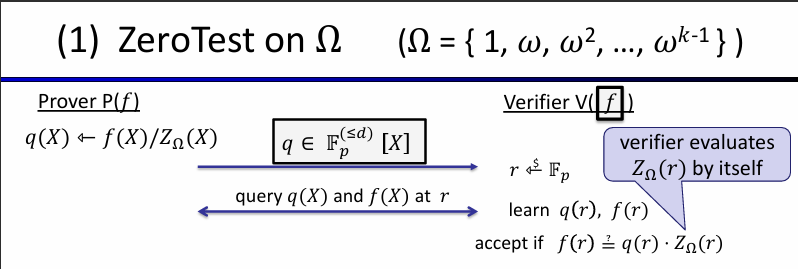
Because $V$ need to evaluate $Z_{\Omega}(r)$ by itself, so we want the vanishing polynomial to be efficiently computable so the verifier can do this quickly. In this situation, our $Z_{\Omega}(r)$ can be calculated fast by square-and-multiply method.
Theorem: This protocol is complete and sound, assuming $\frac{d}{p}$ is negligible
Let’s analyze the costs in this IOP:
For Verifier: $\mathcal{O}(\log k)$ and two poly queries, but can be done in one, thanks to KZG property
For Prover: Dominated by the time to compute $q(X)$ and then commit to $q(X)$
Product Check and Sum Check
Because Prod-check and sum-check are almost identical, so we will only look at prod-check. Again, our claim is that $\prod_{a \in \Omega} f(a) = 1$ and we would like to prove that
Set $t \in \mathbb{F}^{(\le k)}_p[X]$ to be the degree-$k$ polynomial. Define the evaluations of this polynomial as follows:
$t(1) = f(1)$
$t(\omega^s) = \prod_{i=0}^s f(\omega^i), s = 1,..,k-1$
We can notice the recurrence relation between $t$ and $f$: $$ \forall x \in \Omega: t(\omega x) = t(x) f(\omega x)$$ for all $x \in \Omega$ (including at $x = \omega^{k-1}$)
We need a lemma to build this IOP:
Lemma: If $t(\omega^{k-1}) = 1$ and $t(\omega x) - t(x) f(\omega x) = 0$ for all $x \in \Omega$, then $\prod_{a \in \Omega}f(a) = 1$
Let’s write the interactive proof! The idea will to construct another polynomial $t_1(X)$ which is: $$t_1(X) = t(\omega X) - t(x) f(\omega X)$$ which implies that if a zero-test on $t_1(X)$ for $\Omega$ passes, then prod-check passes
Setup: $P$ has a polynomial $f \in \mathbb{F}^{(\le d)} _ p[X], deg(f) = d$ and $V$ has $comm_f$. $V$ wants to prove that $\prod_{a \in Omega}f(a) = 1$
Protocol:
$P$ will constructs $t(X) \in \mathbb{F}_p^{(\le k)}$ and $t_1(X) = t(\omega X) - t(X) f(\omega X)$. The prover also sets $q(X) = t_1(X) / (X^k - 1) \in \mathbb{F}_p^{(\le d)}$ and send $comm_t, comm_q$ to the verifier. Note that $t_1(X)$ should be zero on $\Omega$
The verifier $V$ will choose random $r \in \mathbb{F}_p$, then query $t(X)$ at $\omega^{k-1}, r, \omega r$ to learn $t(\omega^{k-1}), t(r), t(\omega r)$ and query $q(X), f(X)$ at $r$ and $\omega r$ respectively, to learn $q(r)$ and $f(\omega r)$
The verifier will accept if $t(\omega^{k-1}) = 1$ and $t(\omega r) - t(r) f(\omega r) = q(r) (r^k - 1)$
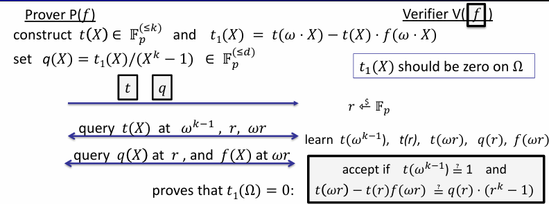
The cost of this protocol is as follows:
Proof size is two commitments $comm_q, comm_t$ and five evaluations. Keeping in mind that evaluations can be batched, the entire proof is just 3 group elements
Prover time is dominated by computing $q(X)$ that runs in time $\mathcal{O}(k \log k)$
Verifier time is dominated by computing $r^k - 1$ and $\omega^{k-1}$, both in time $\mathcal{O}(\log k)
Note that this protocol works for rational functions. Our claim will be $\prod_{a \in \Omega}(f/g)(a) = 1$ and we construct a similar $t$ polynomial, only this time $f(x)$ is divided by $g(x)$ in the definition, then the lemma is also similar: If $t(\omega^{k-1}) = 1$ and $t(\omega x) g(\omega x) - t(x) f(\omega x) = 0$ for all $x \in \Omega$, then $\prod_{a \in \Omega}f(a)/g(a)a = 1$
Permutation Check
Setup:
Let $f, g$ be polynomials in $\mathbb{F}_p^{(\le d)}[X]$. The verifier has $comm_f, comm_g$. Prover wants to prove that:
$(f(1), f(\omega), f(\omega^2),…,f(\omega^{k-1})) \in \mathbb{F}_p^k$
is a permutation of $(g(1), g(\omega), g(\omega^2),…,g(\omega^{k-1})) \in \mathbb{F}_p^k$.
In another way, the prover wants to prove that $g(\Omega)$ is the same as $f(\Omega)$, just permuted
To prove this, we will do what is known as the Lipton’s trick [Lipton'89]. We will construct two auxiliary polynomials:
$\hat{f} = \prod_{a\in \Omega}(X - f(a))$
$\hat{g} = \prod_{a\in \Omega}(X - f(a))$
Then, $g$ is a permutation of $f$ if and only if $\hat{f}(X) = \hat{g}(X)$
Protocol:
The verifier $V$ will choose random $r \in \mathbb{F} _ p$ and send to prover. To prove that $\hat{f} = \hat{g}$, the prover need to show the evaluation of them at point $r$. Calculating these polynomials are a bit expensive, so we can use prod-check on the rational function: $$\frac{\hat{f}(r)}{\hat{g}(r)} = \prod_{a \in \Omega}\frac{r - f(a)}{r - g(a)} = 1$$
If the product is $1$, it means that $\hat{f}(r) = \hat{g}(r)$, and with high probability, $\hat{f} = \hat{r}$
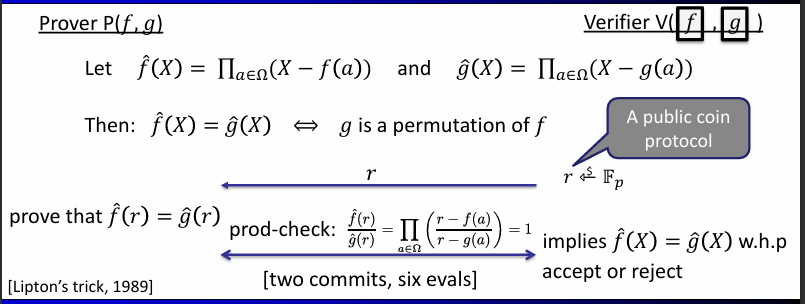
The cost of this proof is just two commitments, and six evaluations
Prescribed permutation check
First, let’s describe the term “permutation” here.
- $W: \Omega \to \Omega$ is a permutation of $\Omega$ if for all $i \in [k]: W(\omega^i) = \omega^j$ is a bijection. For example, with $k = 3$, we will have $W(\omega^0) = \omega^2, W(\omega^1) = \omega^0, W(\omega^2) = \omega^1$
Now, let $f, g$ be polynomials in $\mathbb{F}_p^{(\le d)}[X]$. The verifier has $comm_f, comm_g, comm_W$. The prover wants to prove that $f(y) = g(W(y))$ for all $y \in \Omega$. In another way, $V$ wants to prove that $g(\Omega)$ is the same as $f(\Omega)$, permuted by the prescribed $W$
Why we can’t use a zero-test to prove that $f(y) - g(W(y)) = 0$ on $\Omega$ ? The problem is, the polynomial $f(y) - g(W(y))$ has degree $k^2$, so the prover would need to manipulate polynomials of degree $k^2$. Therefore, we will have quadratic time prover, but our goal is linear time prover.
We can reduce this to a prod-check on a polynomial of degree $2k$. Firstly, let’s talk about the observation that we will use:
Observation: if $(W(a), f(a))_{a \in \Omega}$ is a permutation of $(a, g(a))$ for $a \in \Omega$ , then $f(y) = g(W(y))$ for all $y \in \Omega$
We can prove it by example:
Permutation: $W(\omega^0) = \omega^2, W(\omega^1) = \omega^0, W(\omega^2) = \omega^1$
First set of pairs: $(\omega^0, g(\omega^0)), (\omega^1, g(\omega^1)), (\omega^2, g(\omega^2))$
Second set of pairs: $(\omega^0, f(\omega^0)), (\omega^2, f(\omega^1)), (\omega^1, f(\omega^2))$
Now, we define two auxiliary polynomials, which will be bivariate polynomials of total degree $|\Omega|$:
$\hat{f}(X, Y) = \prod_{a \in \Omega}(X - Y W(a) - f(a))$
$\hat{g}(X, Y) = \prod_{a \in \Omega}(X - Ya - g(a))$
Lemma: $\hat{f}(X, Y) = \hat{g}(X, Y) \iff (W(a), f(a)) _ {a \in \Omega}$ is a permutation of $(a, g(a)) _ {a \in \Omega}$
To proof of this is left as exercise, though if you want to try, you might make use of the fact that $\mathbb{F}_p[X, Y]$ is a unique factorization domain. (I will provide the proof after I learned about UFD :D)
The protocol continues with two random numbers $r, s$ which are chosen by the verifier. To prove that $\hat{f} = \hat{g}$, the prover need to evaluating $\hat{f}, \hat{g}$ at point $(r, s)$. Now, we can use prod-check like permutation check, instead of evaluating the auxiliary polynomials. Our rational function will be:
$$\frac{\hat{f}(r, s)}{\hat{g}(r, s)} = \prod_{a \in \Omega} \Big ( \frac{r - s W(a) - f(a)}{r - s a - g(a)} \Big ) = 1$$
- Therefore, by Schwartz-Zippel lemma, we can conclude that they are equal as bivariate polynomials
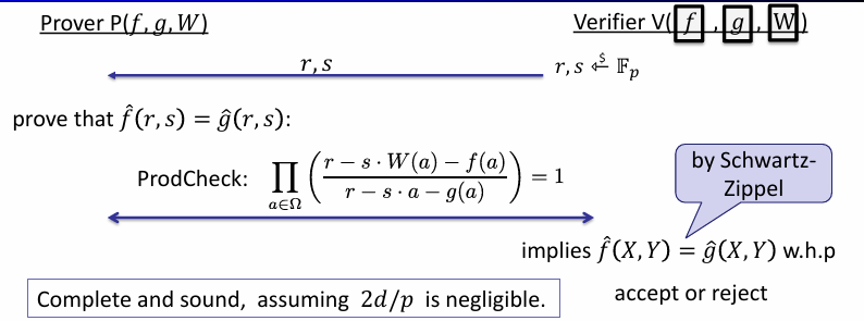
This protocol is sound and complete, assuming $2d/p$ is negligible. The cost of this protocol is just like the cost described for prod-check.
Summarize
Note that our protocols is public-coin protocol, so we can transform our protocols into non-interactive by Fiat-Shamir method.
The PLONK IOP for general circuit
PLONK is a poly-IOP for a general circuit $C(x, w)$
PLONK is widely used in practice, some examples are listed in this table
| Polynomial Commitment Scheme | SNARK System |
|---|---|
| KZG'10 (pairing) | Aztec, JellyFish |
| Bulletproofs (no pairings) | Halo2 (slow verifier but no trusted setup) |
| FRI (hashing) | Plonky2 (no trusted setup) |
Step 1: Compile circuit to computation trace
We will use an example circuit with an example evaluation. Our circuit have gates with two inputs and a single input
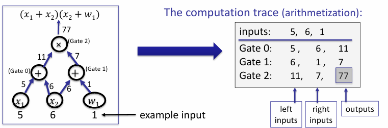
The circuit above computes $(x_1 + x_2)(x_2 + w_1)$. The public inputs are $x_1 = 5, x_2 = 6$ and the secret input (witness) is $w_1 = 1$. We can easily compute the output is $77$, which is also public. The prover will try to prove that he knows a value of $w_1$ that makes the output $77$ with the given public inputs.
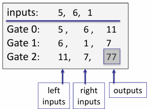
We compile this evaluation into a computation trace, which is simply a table that shows inputs and outputs for each gate, along with circuit inputs.
Circuit inputs are $5, 6, 1$
Gate traces are given in the following table.
Step 1.5: Encode trace as a polynomial
We will define some notations before start:
$|C|$ is the circuit size, equal to number gates in the circuit
$|I| = |I_x| + |I_w|$ is the number of inputs to the circuit, which is the number of public inputs and the secret inputs combined
$d = 3 \times |C| + |I|$
$\Omega = \lbrace 1, \omega, \omega^2, …, \omega^{d - 1} \rbrace$ where $\omega^d = 1$
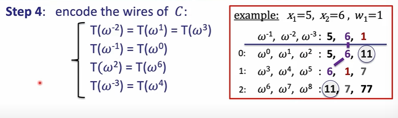
Our plan is interpolates $T \in \mathbb{F}_p^{(\le d)}[X]$ such that
T encodes all inputs: $T(\omega^{-j}) = input_j$ for $j = 1,…,|I|$
T encodes all wires: For all $l = 0, …, |C| - 1$, we have
$T(\omega^{3l})$: left input to gate #l
$T(\omega^{3l + 1})$: right input to gate #l
$T(\omega^{3l + 2})$: output of gate #l
In out example, prover interpolates $T(X)$ such that:
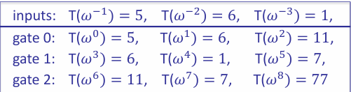
So, our polynomial will have degree 11, and prover can use FFT to compute the coefficients of $T$ in time $\mathcal{O}(d \log d)$
Step 2: Prove validity of $T$
After built $T(X) \in \mathbb{F}_p^{(\le d)}[X]$, the prover send $comm_T$ to the verifier. Now, the verifier must make sure that $T$ indeed belongs to the correct computation trace. To do that, it must do the following:
$T$ encodes the correct inputs
Every gate is evaluated correctly
The “wiring” is implemented correctly
The output of last gate is 0. Well, in this example the output is $77$, but generally the verifier expects a $0$ output.
(1): $T$ encodes the correct inputs
Both prover and verifier interpolate a polynomial $v(X) \in \mathbb{F}_p^{(\le |I_x|)}[X]$ that encodes the $x$-inputs to the circuit: for $j = 1,…,|I_x|$, $v(\omega^{-j}) = input_j$
Next, they will agree on the points encoding the input $\Omega_{inp} = \lbrace \omega^{-1}, \omega^{-2}, …, \omega^{-|I_x|} \rbrace$. Prover proves (1) by using a ZeroTest on $\Omega_{inp}$ to prove that:
$$T(y) - v(y) = 0, \forall y \in \Omega_{inp}$$
(2): Every gate is evaluated correctly
The idea here is encode gate types using a selector polynomial $S(X)$
We define $S(X) \in \mathbb{F}_p^{(\le d)}[X]$ such that $\forall l = 0, …, |C| - 1$:
$S(\omega^{3l}) = 1$ if gate #l is an addition gate
$S(\omega^{3l}) = 0$ if gate #l is a multiplication gate
Then for all $y \in \Omega_{gates} = \lbrace 1, \omega^3, \omega^6, \omega^9,…, \omega^{3(|C| - 1)}$:
$$ S(y)[T(y) + T(\omega y)] + (1 - S(y))(T(y) \times T(\omega y)) = T(\omega^2 y)$$
Here, $T(y), T(\omega y), T(\omega^2 y)$ are the left input, right input and output respectively. Prover will use a zero-test on the set $\Omega_{gates}$ to prove that $\forall y \in \Omega_{gates}$: $$S(y) \times (T(y) + T(\omega y)) + (1 - S(y))(T(y) \times T(\omega y)) - T(\omega^2 y) = 0$$
(3): The wiring is correct
If you look at the circuit (or the table) you will notice that some outputs become inputs on other gates. Prover will have to prove that this wiring has been done correctly
For that, the wires of $C$ are encoded with respect to their constraints
Now, we define a polynomial $W: \Omega \to \Omega$ that implements a rotation: $$W(\omega^{-2}, \omega^1, \omega^3) = (\omega^1, \omega^3, \omega^{-2}), W(\omega^{-1}, \omega^0) = (\omega^0, \omega^{-1})$$
Lemma: $\forall y \in \Omega: T(y) = T(W(y))$ => wire constraints are satisfied
We can prove this lemma by using a prescribed permutation check
(4): Output of last gate is 0
Proving the last one is easy, just show that $T(\omega^{3|C| - 1}) = 0$.
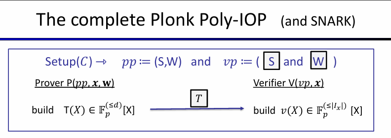
Final step: The PLONK Poly-IOP
Setup: Preprocess the circuit $C$ and outputs $comm_S, comm_W$, which are the selector polynomial $S$ and the wiring polynomial $W$. It is untrusted that everyone can check these commitments were done correctly
Protocol:
Prover $P$ compiles the circuit to a computation trace, and encodes the entire trace into a polynomial $T(X)$
Verifier $V$ can construct $v(X)$ explicitly from the public inputs $x$
Then $P$ proves validity of $T$
gates: evaluated correctly by ZeroTest
inputs: correct inputs by ZeroTest
wires: correct wirings by Prescribed Permutation Check
output: correct output by evaluation proof
Theorem:
The Plonk Poly-IOP is complete and knowledge sound, assuming $7|C|/p$ is negligible
Extension of PLONK
The main challenge is to reduce the prover time.
Hyperplonk: linear prover
Replace $\Omega$ with $\lbrace 0, 1 \rbrace^t$, where $t = \log_2|\Omega|$
The polynomial $T$ is now a multilinear polynomial in $t$ variables
ZeroTest is replaced by a multilinear SumCheck (linear time)
Plonkish Arithmetization: Custom gates and Plonkup
We can use custom gates other than addition gates and multiplication gates. This is used in AIR (Algebraic Intermediate Representation). An example custom gate is: $$\forall y \in \Omega _{gates}: v(y\omega) + v(y)t(y) - t(y\omega) = 0$$
Plonkup enables one to ensure that some values in the computation trace are present in a pre-defined list, basically acting like a look-up argument