Zero Knowledge Proof: Interactive Proofs
Table of Contents
In this post, we will dig deeper about Interactive Proofs, which was described in my previous post.
Resources
ZKP MOOC Lecture 4: Interactive Proofs
Computational Complexity: A Modern Approach, Chapter 8
Detail
Interactive Proofs: Motivation & Model
In an interactive proof, there are two parties: a prover $P$ and a verifier $V$
$P$ solves problem, then tell $V$ the answer
Then they start a conversation, and the goal of $P$ is convince $V$ the answer is correct
There are some requirements for interactive proof
Completeness: an honest $P$ can convince $V$ that the answer is correct
(Statistical) Soundness: $V$ will catch a lying $P$ with high probability. This must hold even if $P$ is computationally unbound and trying to trick $V$ into accept incorrect answer
If soundness holds only against polynomial-time provers, then the protocol is called an interactive argument
Soundness & Knowledge Soundness
We will compare soundness and knowledge soundness for circuit-satisfiability
Let $C$ be some public arithmetic circuit $$C(x, w) \to \mathbb{F}$$ where $x \in \mathbb{F}^n$ is some public statement and $w \in \mathbb{F}^m$ is some secret witness. Let us look at the types of “soundness” with this example:
Soundness: $V$ accepts $\implies \exists w: C(x, w) = 0$
Knowledge Soundness: $V$ accepts $\implies P \ {“knows”} \ w: C(x, w) = 0$
Therefore, we can see that knowledge soundness is stronger, because the verifier must know witness
But standard soundness is meaningful even in contexts where knowledge soundness isn’t, an example is $P$ claims the output of $V$’s program on $x$ is 42. Knowledge soundness isn’t meaningful at below example because there’s no natural witness
Vice-versa, knowledge soundness is meaningful in contexts where standard soundness isn’t. For example, $P$ claims to know the secret key that controls a certain bitcoin wallet. In this one, there does exist a private key to that account for sure, so if using soundness, the verifier can just ignore the verifier and accept, but when using knowledge soundness, $P$ must know the witness
SNARK’s that don’t have knowledge soundness are called SNARGs, and they are studied too!
Public Verifiability
Interactive proofs and arguments only convince the party that is choosing/sending the random challenges, and this is bad if there are many verifiers, cuz the prover would have to convince each verifier separately
To deal with this problem, we can use Fiat-Shamir Transform Fiat, Shamir 87’ to makes the protocol non-interactive and publicly verifiable
In summary
| SNARKs | Interactive Proofs |
|---|---|
| Non-interactive | Interactive |
| Computationally Secure (?) | Information Theoretically Secure (aka Statistically Secure) |
| Knowledge Sound | Not necessary need Knowledge Sound |
SNARKs from interactive proofs: outline
Recall: The trivial SNARK is not a SNARK
(a) Prover sends $w$ to verifier
(b) Verifier checks if $C(x, w) = 0$
Problems with this:
(1) $w$ might be long: we want a “short” proof
(2) Computing $C(x, w)$ maybe hard: we want a “fast” verifier
SNARKs from Interactive Proofs (IPs)
Slight less trivial: $P$ sends $w$ to $V$, and uses an IP to prove that $w$ satisfies the claimed property
- Fast $V$, but proof is still too long
Actual SNARKs
What actually happens in SNARKs is that, instead of sending $w$ explicitly, the prover will cryptographically commit to $w$ and send that commitment.
$P$ uses an IP to prove that $w$ satisfies the claimed property
The prover will reveal just enough information about the committed witness $w$ to allow $V$ to run its checks in the IP
The proof can be made non-interactive using Fiat-Shamir transform
Review of functional commitments
From previous lecture, we had talked about three important functional commitments
Polynomial commitments: commit to a univariate $f(X)$ in $\mathbb{F}_p^{(\le d)}[X]$
Multilinear commitments: commit to multilinear $f$ in $\mathbb{F}_p^{\le 1}[X_1,…,X_k]$
Vector commitments (e.g. Merkle Trees): commit to $\overrightarrow{c} = (u_1,…u_d) \in \mathbb{F}_p^d$
Now, we will discuss more about each one of them
Merkle Trees: The commitment
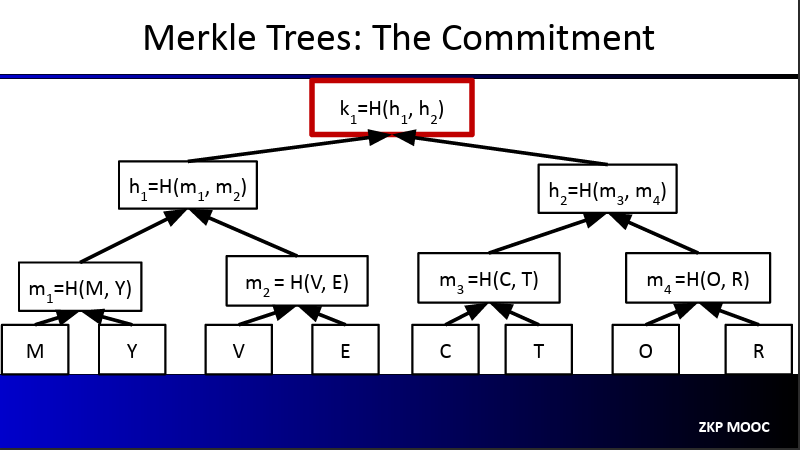
In this binary tree, every node is made up of the hash of its children:
m1 = H(M, Y)h2 = H(m3, m4)k1 = H(h1, h2)
The root k1 is the commitment to this vector
When the prover is asked to show that indeed some element of the vector exists at some position, it will provide only the necessary nodes.
For example, a verifier could ask “is there really a t as position 6?”. The prover will give c, t, h7 and h2 and the verifier will calculate m4, h1, k1. Then, the verifier will compare the calculate h1 to the root given as a commitment by the prover. If they match, then t is indeed at that specific position in the committed vector
Summary, we have:
Commitment to vector is root hash
To open an entry of the committed vector (leaf of the tree):
Send sibling hashes of all nodes on root-to-leaf path
$V$ checks these are consistent with the root hash
“Opening proof” size is O(log n) hash values
Binding: one the root hash is sent, the committer is bound to a fixed vector
- Opening any leaf to two different values requires finding a hash collision (assumed to be intractable)
A First Polynomial commitment: commit to a univariate f(X) in $\mathbb{F}_7^{\le d}[X]$
Suppose that we have a polynomial $f(x) \in \mathbb{F}_7^{\le d} [X]$, so this polynomial has values defined onver a very small $n = 7$. The degree should be small too, say something like $d = 3$
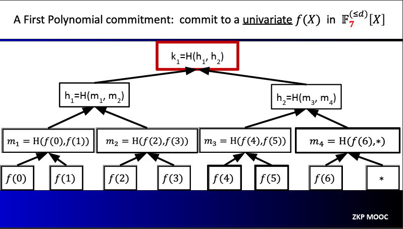
$P$ Merkle-commits to all evaluations of the polynomial $f$
When $V$ requests $f(r)$, $P$ reveals the associated leaf along with opening information
There exists two problems in this method:
The number of leaves is $|\mathbb{F}|$, which means the time to compute the commitment is at least $|\mathbb{F}|$
- Big problem when working over large fields (say, $|\mathbb{F}| \approx 2^{64}$ or $|\mathbb{F}| \approx 2^{128}$)
$V$ does not know if $f$ has degree at most $d$
We will see ways to solve these problems within the lecture
Interactive proof design: Technical preliminaries
Recap: SZDL Lemma
Fact: Let $p \ne q$ be univariate polynomials of degree at most $d$. Then $Pr_{r \in \mathbb{F}}[p(r) = q(r)] \le \frac{d}{|\mathbb{F}|}$
The Schwarts-Zippel-Demillo-Lipton lemma is a multivariate generalization:
Let $p \ne q$ be a $l$-variate polynomials of total degree at most $d$. Then $Pr_{r \in \mathbb{F}^l[p(r) = q(r)]} \le \frac{d}{|\mathbb{F}|}$
“Total degree” refers to the maximum sum of degrees of all variables in any term. E.g., $x_1^2 x_2 + x_1 x_2$ has total degree 3
Low-Degree and Multilinear Extensions
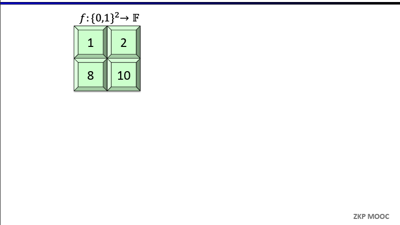
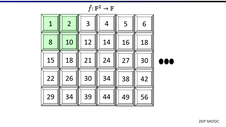
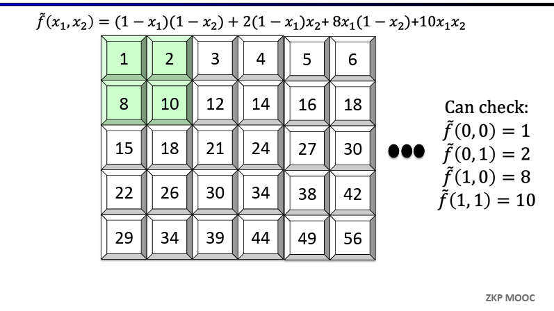
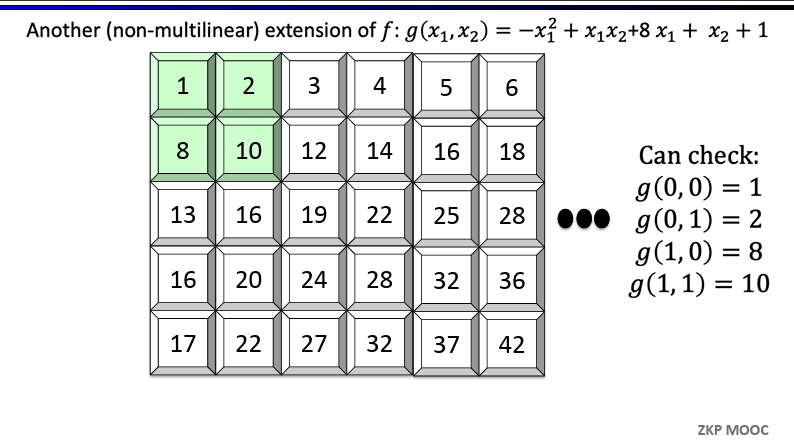
Definition [Extension]. Given a function $f:{0, 1}^l \to \mathbb{F}$, a $l$-variate polynomial $g$ over $\mathbb{F}$ is said to extend $f$ if $f(x) = g(x)$ for all $x \in {0, 1}^l$
Definition [Multilinear Extensions]. Any function $f:{0, 1}^l \in \mathbb{F}$ has a unique multilinear extension (MLE), denoted $\tilde{f}$
Multilinear means the polynomial has degree at most 1 in each variable
$(1 - x_1)(1 - x_2)$ is multilinear, $x_1^2x_2$ is not
Evaluating multilinear extensions quickly
Given as input all $2^l$ evaluations of a function $f: {0, 1}^l \to \mathbb{F}$, for any point $r \in \mathbb{F}^l$ there is an $\mathcal{O}(2^l)$-time algorithm for evaluating the MLE $\tilde{f}(r)$
We will use Lagrange Interpolation. For every input $\omega = (\omega_1, \omega_2,…,\omega_l) \in {0, 1}^l$, define the multilinear Lagrange Basis polynomial as follow $$\tilde{\delta} _ {\omega}(r) = \prod _ {i=1}^{l}(r_i\omega_i + (1 - r_i)(1 - \omega_i))$$
So we can get the evaluation of $\tilde{f}(r)$ using these: $$f(r) = \sum _ {\omega \in \lbrace 0, 1 \rbrace^l}f(\omega) \times \tilde{\delta} _ {\omega}(r)$$
For each $\omega \in {0, 1}^l$, the result $\tilde{\delta} _ {\omega}(r)$ can be computed with $\mathcal{O}(l)$ field operations. As such, the overall algorithm for $2^l$ points takes time $\mathcal{O}(l2^l)$. Using dynamic programming, this can be reduced to $\mathcal{O}(2^l)$
The sum-check protocol
We are going to work with the sum-check protocol Lund-Fortnow-Karloff-Nissan'90.
The verifier $V$ given oracle access to a $l$-variate polynomial $g$ over field $\mathbb{F}$, and the goal of $V$ is compute the quantity: $$\sum _{b_1 \in \lbrace 0, 1 \rbrace} \sum _ {b_2 \in \lbrace 0, 1 \rbrace} … \sum _ {b_l \in \lbrace 0, 1 \rbrace} g(b_1, b_2,…,b_l)$$
In the naive method, the verifier would query each input, and find the sum in a total of $2^l$ queries. We will consider this to be a costly operation
Instead, a prover will compute the sum and convince a verifier that this sum is correct. In doing so, the verifier will make only a single query to the oracle! Let’s see how. Denote $P$ as prover and $V$ as verifier
- Start: $P$ sends the claimed answer $C_1$. The protocol must check that indeed:
$$C_1 = \sum _ {b_1 \lbrace 0, 1 \rbrace} \sum _ {b_2 \lbrace 0, 1 \rbrace} … \sum _ {b_l \lbrace 0, 1 \rbrace} g(b_1, b_2,…,b_l)$$
- Round 1: $P$ sends univariate polynomial $s_1(X_1)$ claimed to equal $H_1(X_1)$ (H standing for honest):
$$H_1(X_1) = \sum _ {b_1 \lbrace 0, 1 \rbrace} \sum _ {b_2 \lbrace 0, 1 \rbrace} … \sum _ {b_l \lbrace 0, 1 \rbrace} g(X_1, b_2,…,b_l)$$
– $V$ need to check two things:
Does $s_1$ equal $H_1$ ?
If $s_1$ does equal $H_1$, is that consistent with the true answer being $C_1$ ?
– For the second question, the verifier simply checks that $C_1 = s_1(0) + s_1(1)$. If this check passes, it is safe for $V$ to believe that $C_1$ is the correct answer, so long as $V$ believes that $s_1 = H_1$
– For the first question, $V$ just check that $s_1$ and $H_1$ agree at a random point $r_1$
– Remember that, $V$ can compute $s_1(r_1)$ directly from $P$’s first message, but not $H_1(r_1)$
Round 2: They recursively check that $s_1(r_1) = H_1(r_1)$. i.e., that $$s_1(r_1) = = \sum _ {b_2 \lbrace 0, 1 \rbrace} … \sum _ {b_l \lbrace 0, 1 \rbrace} g(r_1, b_2,…,b_l)$$
Recursion into Rounds 3,4,…,$l$: The verifier and prover keep doing this until the last round
Final Round (Round $l$): $P$ sends univariate polynomial $s_l(X_l)$ claimed to equal $$H_l := g(r_1,…,r_{l-1}, X_l)$$
– $V$ checks that $s_{l-1}(r_{l-1}) = s_l(0) + s_l(1)$
– $V$ picks $r_l$ at random, and needs to check that $s_l(r_l) = g(r_1,…,r_l)$
- The verifier doesn’t need for more rounds, because $V$ can perform this check with one oracle query
Analysis of the sum-check protocol & costs
Completeness: It holds by design: If $P$ sends the prescribed messages, then all of $V$’s checks will pass
Soundness: If $P$ does not send the prescribed messages, then $V$ rejects with probability at least $1 - \frac{ld}{| \mathbb{F} |}$, where $d$ is the maximum degree of $g$ in any variable. You can proof by induction on the number of variables $l$
Total communication is $\mathcal{O}(dl)$ field elements
$P$ sends $l$ messages, each a univariate polynomial of degree at most $d$. $V$ sends $l - 1$ messages, each consisting of one field element
$V$’s runtime is: $$\mathcal{O}(dl + [time \ required \ to \ evaluate \ g \ at \ one \ point])$$
$P$’s runtime is at most: $$\mathcal{O}(d * 2^l * [time \ required \ to \ evaluate \ g \ at \ one \ point])$$
Application: Counting Triangles in a graph
Input: $A \in \lbrace 0, 1 \rbrace^{n \times n}$, representing the adjacency matrix of a graph
Desired Output: $\sum_{(i, j, k) \in [n]^3} A_{ij}A_{jk}A_{ik}$
The Protocol:
View $A$ as a function mapping ${0, 1}^{\log n} \times {0, 1}^{\log n}$ to $\mathbb{F}$
Recall that $\tilde{A}$ denotes the multilinear extension of $A$
Define the polynomial $g(X, Y, Z) = \tilde{A}(X, Y) \tilde{A}(Y, Z) \tilde{A}(X, Z)$
Apply the sum-check protocol to $g$ to compute $$\sum_{(a, b, c) \in \lbrace 0, 1 \rbrace ^{3 \log n}} g(a, b, c)$$
Costs:
Total communication is $\mathcal{O}(\log n)$, $V$ runtime is $\mathcal{O}(n^2)$, $P$ runtime is $\mathcal{O}(n^3)$
$V$’s runtime dominated by evaluating: $$g(r_1, r_2, r_3) = \tilde{A}(r_1, r_2) \tilde{A}(r_2, r_3) \tilde{A}(r_1, r_3)$$
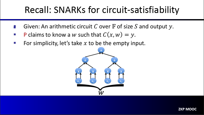
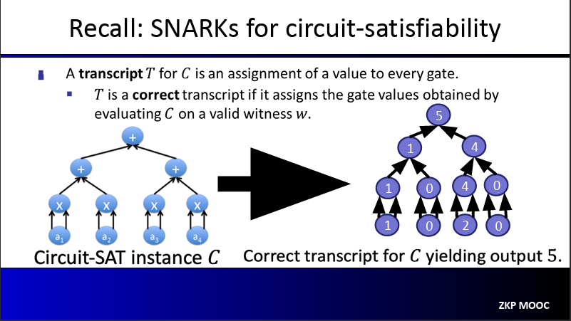
A SNARK for circuit-satisfiability
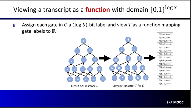
We will use a notion of transcript, which is defined as an assignment of a value to every gate in the circuit. A transcript $T$ is a correct transcript if it assigns the gate values obtained by evaluating the circuit $C$ on a valid witness $\omega$
The polynomial IOP underlying the SNARK
Recall that our SNARK is all about proving that we know a secret witness $\omega$ such that for some public input $x$ and arithmetic circuit $C$ it holds that $C(x, \omega) = 0$. Denote the circuit size as $S = |C|$
First, we will construct the correct transcript of $C(x, \omega)$, which we denote as $T: {0, 1}^{\log S} \to \mathbb{F}$.
Prover $P$ will calculate the extension of $T$ to obtain a polynomial $h: \mathbb{F}^{\log S} \to \mathbb{F}$. This extension $h$ is the first message sent to the verifier $$\forall x \in \lbrace 0, 1 \rbrace^{\log S}: h(x) = T(x)$$
The verifier $V$ needs to verify that this is indeed true, but it will only make a few evaluations of $h$ in doing so
The intuition behind using extensions is that: If there is even just a singe tiny error in the transcript, so by Schwartz-Zippel theorem,the extension of this transcript will disagree on almost all points with respect to the correct transcript.
Step 1:
Given $(\log S)$-variate polynomial $h$, identify a related $(3 \log S)$-variate polynomial $g_h$ such that: $h$ extends a correct transcript if and only if $g_h(a, b, c) = 0 \forall (a, b, c) \in {0,1}^{3 \log S}$ and to evaluate $g_h(r)$ at any $r$, suffices to evaluate $h$ at only 3 inputs
So, we will define $g_h(a, b, c)$ via: $$\tilde{add}(a, b, c)(h(a) - (h(b) + h(c))) + \tilde{mult}(a, b, c) (h(a) - h(b)h(c))$$
Let’s just quickly introduce what the functions $\tilde{add}$ and $\tilde{mult}$ are:
$\tilde{add}(a, b, c)$ is a multilinear extension of a wiring predicate of a circuit, which return 1 if and only if $a$ is an addition gate and it’s two inputs are gates $b$ and $c$
$\tilde{mult}(a, b, c)$ is a multilinear extension of a wiring predicate of a circuit, which returns 1 if and only if $a$ is a multiplication gate and it’s two inputs are gates $b$ and $c$
With the definition, we can see what happens:
$g_h(a, b, c) = h(a) - (h(b) + h(c))$ if $a$ is the label of a gate that computes the sum of gates $b$ and $c$
$g_h(a, b, c) = h(a) - h(b)h(c)$ if $a$ is the label of a gate that computes the product of gates $b$ and $c$
$g_h(a, b, c) = 0$ otherwise
Step 2:
How can the verifier check that indeed $\forall (a, b, c) \in {0,1}^{3 \log S}: g_h(a, b, c) = 0$ ? In doing so, verifier should only evaluate $g_h$ at a single point!
We will use a well-known result in polynomials: $\forall x \in H: g_h(x) = 0 \iff Z_h(x) | Z_H(x)$, where $Z_H(x)$ is called the vanishing polynomial for $H$ and is defined as: $$Z_H(x) = \prod_{a\in H}(x - a)$$
Then, the polynomial IOP will work as follows:
$P$ sends a polynomial $q$ such that $g_h(X) = q(X) \times Z_H(X)$
$V$ verifies this by picking a random $r \in H$ and checking $g_h(r) = q(r) \times Z_H(r)$
In realworld, this approach is not really the best approach because of it’s problems
$g_h$ is not univariate, it has $3 \log S$ variables
Having $P$ find and send the quotient polynomial is expensive
In the final SNARK, this would mean applying polynomial commitment to addition polynomials.
Although it has some problems, but this approach is actually used by well-known schemes: Marlin, PlonK and Groth16 do
To deal with that problems, we can use the sum-check protocol: It handles multivariate polynomials, and doesn’t require $P$ to send additional large polynomials
Here is the general idea (We are working over the integers instead of $\mathbb{F}$):
$V$ checks this by running sum-check protocol with $P$ to compute: $$\sum_{a, b, c \in \lbrace 0, 1 \rbrace^{\log S}}g_h(a, b, c)^2$$
If all terms in the sum are 0, the sum is 0
If working over the integers, any non-zero term in the sum will cause the sum to be strictly positive
At end of sum-check protocol, $V$ needs to evaluate $g_h(r_1, r_2, r_3)$
Suffices to evaluate $h(r_1), h(r_2), h(r_3)$, because $V$ will only compute $g_h(r_1, r_2, r_3)$ for some random inputs.
Outside of these evaluations, $V$ runs in time $\mathcal{O}(\log S)$
$P$ performs $\mathcal{O}(S)$ field operations given a witness $\omega$
To understand more about the polynomial IOP, I suggest reading Justin Thaler’s online book, chapters 3 and 4, which is noticed at the resources section.